> For the complete documentation index, see [llms.txt](https://thesis.duarteocarmo.com/llms.txt). Markdown versions of documentation pages are available by appending `.md` to page URLs; this page is available as [Markdown](https://thesis.duarteocarmo.com/new-part/quantitative-analysis.md).
# Quantitative Analysis
In this fourth and final section of the methodology chapter, several quantitative analysis techniques will be introduced. Some of the concepts described in this section are based on literature that was covered in the second chapter; others were developed especially in the scope of this project.
## Normalizations
During the analysis, several measures had to be normalized in order to focus on patterns rather than volume of occurrence. For example, the United States of America is the country that produces the most patents in the world and therefore, if one wants to compare its capability matrix to the capability matrix of another country, the results should be normalized:
Let us define the normalized capability matrix as:
`Bijk=AijkNk ∀i,j, k`
Where, Aijk is the capability matrix of a certain category k, Bijk the normalized capability matrix of that same category, and Nk the total number of technological assets owned by or located in that category.
Another important normalization is related to the chronological evolution of records. There is a tendency for an increase in the number of technological assets over time, and therefore if the study is focused on the proportion of technological assets of a particular type in a year, a normalization should also be applied:
`TNormk= TAbskNk`
Where TNormk is the normalized number of records in k, TAbsk is the absolute number of records in k, and Nk the total number of records in that period k.
## Capability Matrix Operations
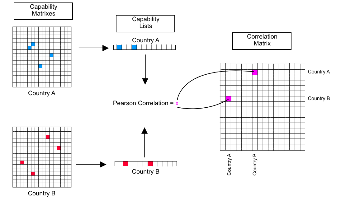
The second important quantitative analysis operation is related to comparing capability matrices of different entities. In order to compare two or more capability matrices, a python script was developed to transform a capability matrix into a list.

This script takes all of the unique values of a capability matrix (58482) and places them in a vector with a total of 58482 entries which will be referred to as a capability list.
In order to compare two capability matrices, the first step is to create two capability lists, after doing this, the Pearson correlation index was chosen as an indicative of the similarity between them.
## Correlation Matrix
Another important concept when comparing capability matrixes is the concept of a correlation matrix.
When comparing units (countries, years, organizations), in order to understand how there capability matrices differ, the Pearson correlation index was used (as above described). Let us say that there are a total of 100 countries to compare. By comparing every country to each other, a correlation matrix between all of the countries can be created. The figure below illustrates this concept.
## Hierarchical Clustering
In order to find the clusters of entities whose capability matrices are more similar and consequently find “capability groups” the main technique used derives from unsupervised learning: hierarchical clustering. This method seeks to form a hierarchy of clusters from data points and is usually expressed through a dendrogram of connections.
This method was applied by the use of the [scipy](https://www.scipy.org/) python library which also allows for the determination of a particular hierarchical clustering method. A hierarchical clustering method is usually defined by the distance measurement that helps in building clustering, such measures include: ward, single, complete, average. Through trial and error, it was determined that the average distance method was the most appropriate for the analysis.
## Collaboration
Another important measure that was used throughout the analysis is the relationship between countries, universities or organizations. To quantify this measure, as previously described in the triple-helix framework in the literature review, the properties of the graph database were used.
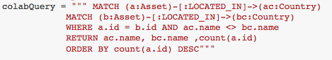
Using the cypher language, it is possible to retrieve technological assets that are located (in the case of countries), or owned by (in the case of organizations), by two different entities. For instants, when comparing France and Denmark, if the query above returns 45 documents, this means that France and Denmark collaborated in 45 different technological assets. The same logic applies to organizations.
## External data and considerations
Throughout the analysis, several external data was used, mainly for considerations regarding the relationship between these externalities and the patterns detected in the data treated.
The first data was the Gross Domestic Product (GDP), extracted from the World Data Bank ([link](https://data.worldbank.org/indicator/NY.GDP.PCAP.CD)). This indicator was extensively used in national innovation studies previously mentioned in the literature review, and serves as comparative index of economic development between two countries. However, in order to preserve the scale of the analysis, the GDP per capita was used. Moreover, the GDP per capita average and difference of country pairs was also used. Since only considering the GDP per capita difference could provide a too “simplistic” analysis, the GDP per capita average gives information about the relative richness of the country pair, and not only how different the two countries are. On a second note, the analysis also sought to relate chronological development of certain technological assets with the evolution of external factors, in order to understand their intricate relationship (if there is one). As a proof of concept, two indexes were used, a more general one and a more specific one. The more general index, price per gallon of oil ([link](https://fred.stlouisfed.org/series/GASREGCOVM#0)) in $US, and the more specific index, price per kg of sugar ([link](http://databank.worldbank.org/data/home.aspx?access=N)). In the introductory part of the analysis, their evolution over time is compared to the usage of specific terms as a possible way of understanding the behavior of the biofuel research landscape.