> For the complete documentation index, see [llms.txt](https://thesis.duarteocarmo.com/llms.txt). Markdown versions of documentation pages are available by appending `.md` to page URLs; this page is available as [Markdown](https://thesis.duarteocarmo.com/new-part/network-model.md).
# Network Model
## Model Criteria
In the third part of the chapter, the focus will lie in the description of the engineering systems representation that was developed. The developed model would have to respect a number of important criteria:
* Accurately portray the biofuel research landscape dynamics.
* Preserve the complexity of term combinations. Simply describing the frequency of a certain term throughout documents would not be enough.
* Be scalable to different dimensions, particularly the global level, the country level and the organizational level.
* Statistical analysis and pattern detection should be possible in order to detect patterns and answer quantitative questions.
One possible way of respecting these constraints with the available data goes back to the graph/network system approach. As previously stated, one of the advantages of this approach relies in the visualization and statistical analysis of a particular system. But the graph system approach is not per se a mathematical definition of how a system should be expressed; however, one of the possibilities that appear in the literature is the creation of a matrix that expresses the frequency of pair combinations.
## Adjacency Matrix
An adjacency matrix is a mathematical term that seeks to express a network through a matrix. Let us mathematically define it as:
`Aij=x`
* The value of x is equal to 0 if node i and j are not connected.
* The value of x is proportional to the weight of the edge between node i and node j.
The adjacency matrix is purely symmetrical:
`Aij=Aji ∀i,j`
In this case, the connection of a node with itself is discarded, therefore the diagonal of the adjacency matrix is equal to zero if a:
`Aij=0 ∀i,j:i=j`
## Model
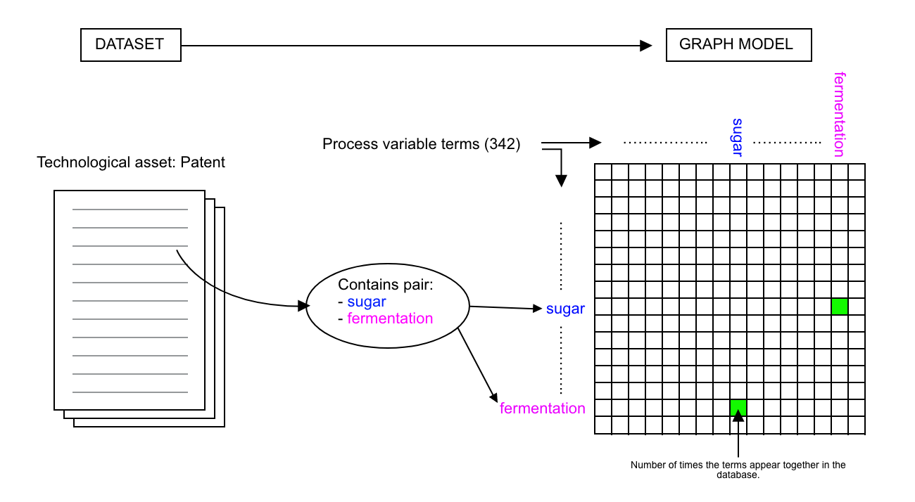
The model proposed is based on the adjacency matrix; it treats every term (feedstock, output, processing technology) as a node in the network. If two terms appear in the same document, then these nodes are connected. The weight of the edge connecting these nodes is proportional to the number of times that these appear together throughout the database. For example, let us say that “fermentation” and “corn” appear together in assets 45 times in a database, then, the edge that connects them will have a weight of 45.
In the model, the rows and columns of the matrix are all of the process variable terms that exist in the database (in total 342 distinct terms). Which will create a 342x342 adjacency matrix, with a total of 116964 values, of which 58 482 are unique (due to symmetry).
A graphical representation follows:
This graph model is highly powerful not only because of its capacity to capture all of the pairwise combinations of terms but also because of its scalability. In fact, one can apply this model to several levels of the analysis by pre-filtering the technological assets used to build the adjacency matrix.
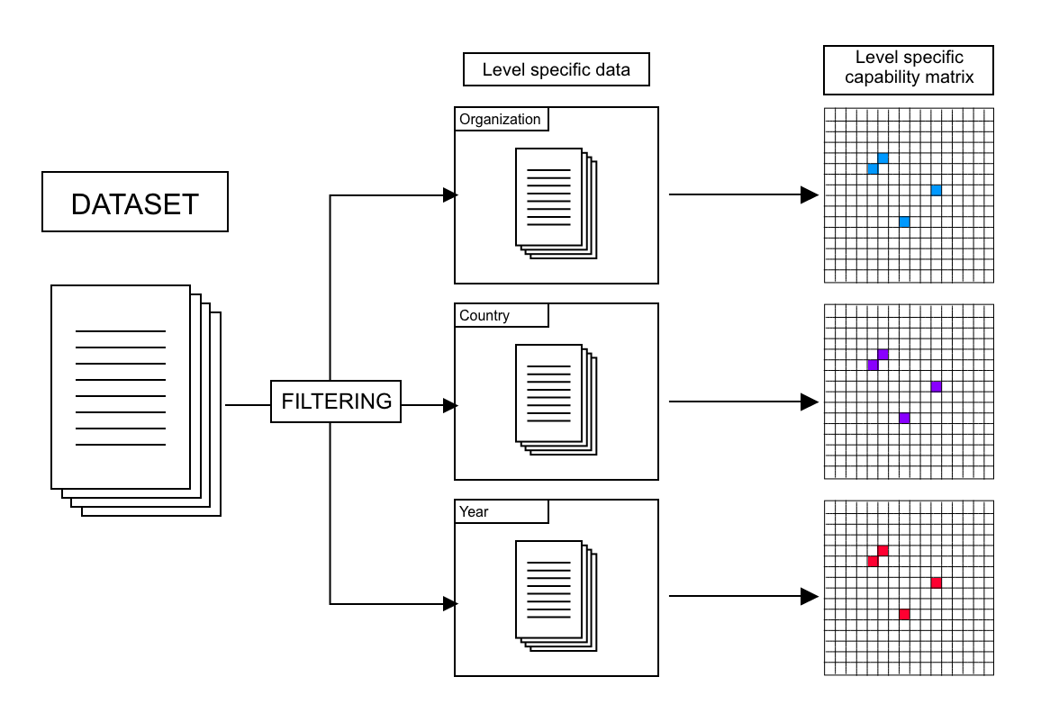
If only documents from a particular year, country, or organization serve as input, then the subsequent model will represent the technological capability of that particular unit, or its capability matrix. It is important to note that whatever the filtering (per organization, per country) applied to the data, the capability matrix will always have the same dimensions; this is because the extraction of all of the process variable terms was made beforehand. This allows the application of the same quantitative analysis techniques to all of the levels of the project.
Finally, looking back at the graph model constraints established at the beginning of the section, it can be said that this model appears to respect them entirely. By representing the entirety of term pairs used across documents, it not only represents the research landscape, but also preserves the scientific complexity of such research. Moreover, the pre-filtering of documents allows for scalability of the model, and the fixed matrix structure allows for the quantitative analysis.